Together with my friend and former colleague Georgios Kaiafas, we formed a team to participate to the Athens Datathon 2015, organized by ThinkBiz on October 3; the datathon took place at the premises of Skroutz.gr, which was also the major sponsor and the data provider. It was the second such event organized in Athens, and you can see the Datathon 2014 winner team’s infographic here.
Skroutz is the leading platform in Greece for online price comparison, and they have recently started business in Turkey and the UK, too. The dataset they provided for the datathon consisted of 30 log files, one for each day of September 2013, along with a file with some elementary demographic information of their registered users; needless to say, all user data were anonymized.
Specific predefined objectives for the Datathon had not been set; the general requirement, quite understandably, was simply “impress us!”, by finding something of business value and present it in an appropriate way.
Our participation to the Datathon, apart from fun, was also of great value, both for me and Georgios, for various reasons that I hope to make clear in this post; I am going to undertake a more or less chronological narrative, aiming to offer some insight into how a data exploration process actually works in practice, instead of how it is viewed after the fact, possibly as part of a finished project report.
So, let’s get introduced to the datasets provided…
(Note: All work presented here is the common result of collaboration between me and Georgios; his favorite data analysis tool is Python & pandas, while mine is R and the fabulous data.table package. Since the post happens to be written by myself, only R code will be shown here; nevertheless, we hope to make available the equivalent Python code in Github, soon UPDATE: Python code by Georgios is now on Github).
Getting familiar with the data
Contrary to what seemed to happen with many other teams using different tools, loading the data with Python/pandas or R was completely straightforward. Let’s have a look at the users data first:
> library(data.table)
data.table 1.9.4  For help type: ?data.table
*** NB: by=.EACHI is now explicit. See README to restore previous behaviour.
> users <- fread('c:/datathon/user_info.csv', header=FALSE)
> names.users <- c('id', 'registration.date', 'registration.type', 'sex', 'DOB')
> setnames(users, names.users)
> head(users)
                                         id         registration.date registration.type  sex        DOB
1: 5f183c75ae05809c7a032086d00a96dbfb2e20d3 2006-11-18 03:00:01 +0200                 0
2: a403461d184f687966e81b17ccac6a13aebca1aa 2006-11-18 03:00:01 +0200                 0
3: 384b411b1e0d5a85987fce29cf269f225c677f71 2006-11-18 03:00:01 +0200                 0 male 1988-01-01
4: 7e5319d97b4efe14d87007681530949d883732ec 2006-11-18 03:00:01 +0200                 0 male 1976-01-01
5: 6de81938fb6b49dbbe27aa67a7253cb90e622499 2006-11-18 03:00:01 +0200                 0 male 1975-01-01
6: a33c5bd9e1f165367bc75c3b305ef4c030dbb7e6 2006-11-18 03:00:01 +0200                 0 male 1975-01-01
> nrow(users)
[1] 15218
So, we had about 15,000 registered users, with the fields shown above. Observing missing values in attribute sex, we proceeded to check for how many users we actually had gender information; but before doing so, let me warn you that I am a fan of the magrittr R package and the pipe (%>%) operator, which Tal Galili, moderator of R-bloggers, has called “one (if not THE) most important innovation introduced, this year [2014], to the R ecosystem” (his emphasis):
> library(magrittr)
> users[sex=='male'] %>% nrow
[1] 6161
> users[sex=='female'] %>% nrow
[1] 1018
So, we had gender info for only about 45% of the registered users, the great majority of which were male.
Next step, to have a look at one log file:
> setwd("C:/datathon/dataset")
> f = '2013_09_01.log'
> df = fread(f, header=FALSE)
> names.df = c('sttp','UserSessionId', 'RegisteredUserId', 'PathURL',
+ 'action', 'Time', 'Query', 'CategoryId', 'ShopId',
+ 'ProductID', 'RefURL', 'SKU_Id','#Results')
> setnames(df,names.df)
> nrow(df)
[1] 330032
> head(df)
sttp UserSessionId RegisteredUserId PathURL action Time Query CategoryId
1: 22 89eca7cf382112a1b82fa0bf22c3b6c0 /search 1377982801.6669302 Ï„Ïαπεζι κουζινας με καÏεκλες
2: 10 edec809dcd22538c41ddb2afa6a80958 /products/show/13160930 1377982802.7676952 12Q420 405
3: 22 333542d43bc440fd7d865307fa3d9871 /search 1377982803.1507218 maybelline
4: 10 df15ec69b3edde03f3c832aa1bba5bed /products/show/9546086 1377982803.4333012 Hugo Boss 790
5: 10 d8b619b5a14c0f5f4968fd23321f0003 /products/show/8912067 1377982804.0093067 xbox 360 109
6: 22 d2a0bb0501379bfc39acd7727cd250e8 9a7950cf6772b0e837ac4f777964523b5a73c963 /search 1377982804.6995797 samsung galaxy s4 mini
ShopId ProductID
1:
2: de12f28477d366ee4ab82fbab866fb9fca157d5c 7c1f7d8ed7c7c0905ccd6cb5b4197280ea511b3e
3:
4: d1c8cad880ecd17793bb0b0460cb05636766cb95 f43f7147a8bf6932801f11a3663536b160235b1f
5: 5149f83f83380531b226e09c2f388bffc5087cbe 550ae3314e949c0a7e083c6b0c7c6c1a4a9d2048
6:
RefURL SKU_Id #Results
1: http://www.skroutz.gr/c/1123/dining_table.html?keyphrase=%CF%84%CF%81%CE%B1%CF%80%CE%B5%CE%B6%CE%B9+%CE%BA%CE%BF%CF%85%CE%B6%CE%B9%CE%BD%CE%B1%CF%82&order_dir=asc&page=2 3
2: http://www.skroutz.gr/s/442786/Siemens-WM12Q420GR.html?keyphrase=12Q420 442786
3: http://www.skroutz.gr/search?keyphrase=maybelline+bb 11
4: http://www.skroutz.gr/s/1932513/Hugo-Boss-0032S.html 1932513
5: http://www.skroutz.gr/c/109/gamepads.html?keyphrase=xbox+360&order_dir=asc&page=11 1475611
6: https://www.skroutz.gr/ 3
All these attributes were described in provided documents, and contest “mentors” were always around, ready to answer questions and clarify things. I will not go through a detailed attribute description here; for our purposes, it suffices to say that the attribute linking the two pieces of data (log files & users info) is RegisteredUserId: that is, in a log entry of a registered user, this attribute is equal to the id attribute of the respective user in the users info file (shown above). For a non-registered user, the attribute in the log is simply missing (e.g. the 5 first values shown above).
At about this point, we thought of focusing to the registered users only, for which gender info was available, so that we could subsequently try to detect possible different patterns in the browsing behavior correlated with difference in gender.
Getting the log actions per registered user gender is straightforward; first, we isolate the respective id’s from users info:
> male.id <- users[sex == "male",id]
> female.id <- users[sex == "female",id]
Afterwards, we can easily get the indices of the male/female actions in the log as follows:
df[,RegisteredUserId] %in% male.id    # indices of registered male users' actions in the log
df[,RegisteredUserId] %in% female.id  # indices of registered female users' actions in the log
All was looking good! We had just a sanity check to do: the number of all log records belonging to (registered) male/female/(blank) users should be equal to the number of records with a non-missing RegisteredUserId attribute.
Only it was not:
> nosex.id <- users[sex == '',id]
> sum(df[,RegisteredUserId] %in% male.id) + sum(df[,RegisteredUserId] %in% female.id) + sum(df[,RegisteredUserId] %in% nosex.id) == nrow(df[RegisteredUserId != ''])
[1] FALSE
What the…
“You’re exaggerating! It’s probably just some glitch during data preparation…”
Sensibly enough, the first thing we thought was that, in the users file, there were possibly different spellings of male/female (e.g. MALE, Female etc), but this proved not to be the case:
> users[,.N, by=sex]
      sex    N
1:        8039
2:   male 6161
3: female 1018
At that point, there was an obvious “usual suspect”: could it be that there were registered users with actions in the logs, which had not been included in the provided users info file?
We posed this question to the datathon mentors; the answer we received was that this should normally not have happened, but, quite understandably, nobody could exclude a glitch during the data preparation phase, leaving “a couple or so of registered customers out of the users info file“…
Only, the excess actions could not likely be attributed to a couple or so “missed” registered users… Let’s see exactly how big the discrepancy was:
> x1 <- sum(df[,RegisteredUserId] %in% male.id)
> x2 <- sum(df[,RegisteredUserId] %in% female.id)
> x3 <- sum(df[,RegisteredUserId] %in% nosex.id)
> x <- x1 + x2 + x3
> x
[1] 9797
> y <- nrow(df[RegisteredUserId != ''])
> y
[1] 13528
> y-x
[1] 3731
So, the case was that, out of 13,500 actions by registered users in the first log file (2013-09-01.log), about 3,700, or 27%, belonged to some “phantom” users which, although registered, had not been included in the users info file.
Yes, such things happen, of course…
By then, we had already started receiving visits from datathon mentors in our working place: it was apparent that we were the only team that had raised such an issue, and, involuntary, we had probably created some amount of “noise”. These visits did not shed any light on our finding – in fact, we even received a friendly (well, kind of…) reminder from one individual that “You know, such issues in the data is something you are expected to deal with“…
Well of course, I couldn’t agree more.
At that point, along with Georgios, we had to come up with a decision, since a) time was passing and b) all our analysis until then was only on the first log file (out of 30 in total):
- either we would continue on our designed path of actions, ignoring the issue, since we could lightheartedly attribute it to some glitch during data preparation (this was the consensus, at least among the datathon mentors who actually believed us)
- or we would keep on drilling, until we were more confident and certain about the exact nature of the issue, but, at the same time, taking the risk of running out of time and finding ourselves with empty hands and nothing to report at the datathon finale
I am really happy and proud that, facing these two options, we did not choose the wrong one…
Homing on the anomaly
OK, it was time to take a closer look at these phantom users – who were they? To speed things up, and since we were not using the log entries of unregistered users, we cleared them up, building a new dataframe df.registered containing only the actions of registered users:
> df.registered <- df[RegisteredUserId != '']
> anom.id <- df.registered[!(RegisteredUserId %in% users[,id]),RegisteredUserId ]
> head(anom.id)
[1] "cdc75a725963530a598e71c70677926b9a5f1bc1" "cdc75a725963530a598e71c70677926b9a5f1bc1" "cdc75a725963530a598e71c70677926b9a5f1bc1"
[4] "cdc75a725963530a598e71c70677926b9a5f1bc1" "cdc75a725963530a598e71c70677926b9a5f1bc1" "cdc75a725963530a598e71c70677926b9a5f1bc1"
> tail(anom.id)
[1] "cdc75a725963530a598e71c70677926b9a5f1bc1" "cdc75a725963530a598e71c70677926b9a5f1bc1" "cdc75a725963530a598e71c70677926b9a5f1bc1"
[4] "cdc75a725963530a598e71c70677926b9a5f1bc1" "cdc75a725963530a598e71c70677926b9a5f1bc1" "cdc75a725963530a598e71c70677926b9a5f1bc1"
> unique(anom.id)
[1] "cdc75a725963530a598e71c70677926b9a5f1bc1"
Oopsss… what was that? One single user? Was it possible? We had probably made some mistake, somewhere… Let’s try a quick sanity check – how many user actions with this particular RegisteredUserId existed in our log file?
> df[RegisteredUserId == 'cdc75a725963530a598e71c70677926b9a5f1bc1'] %>% nrow
[1] 3731
> users[id == 'cdc75a725963530a598e71c70677926b9a5f1bc1'] %>% nrow
[1] 0
(Recall from above that 3731 was exactly the number of excess actions in the log.)
So, we had finally located our phantom: it was just a single one, its name was 'cdc75a725963530a598e71c70677926b9a5f1bc1', and, although registered, it had not allowed itself to be included in the registered users file (but again, which respectable phantom would allow itself to be listed?).
Chasing the phantom
OK, we had discovered a phantom in the first log file; we had only 29 log files left, to see what was happening there. And time was still passing.
But if you know (even roughly) what you are looking for, things are much more straightforward; the following R script reads each log file sequentially and stores the number of anomalies (i.e. actions by registered users that are not themselves included in the users info file) and the specific RegisteredUserId‘s related to these anomalous actions, to the variables anom and anom.id, respectively (highlighted lines):
library(data.table)
library(magrittr)
# read users' info first:
users <- fread('c:/datathon/user_info.csv', header=FALSE)
names.users <- c('id', 'registration.date', 'registration.type', 'sex', 'DOB')
setnames(users, names.users)
# now continue with the log files
setwd("C:/datathon/dataset")
loglist <- list.files()
anom <- rep(0, length(loglist))
anom.id <- list()
names.df = c('sttp','UserSessionId', 'RegisteredUserId', 'PathURL',
               'action', 'Time', 'Query', 'CategoryId', 'ShopId',
               'ProductID', 'RefURL', 'SKU_Id','#Results')
k <- 1
for (f in loglist) {
  df = fread(f, header=FALSE)
  setnames(df,names.df)
  df.registered <- df[RegisteredUserId != '']  # keep only registered users
  anom[k] <- df.registered[!(RegisteredUserId %in% users[,id]) ] %>% nrow  # no of anomalous actions
  anom.id[k] <- df.registered[!(RegisteredUserId %in% users[,id]), RegisteredUserId ] %>% unique # find unique user id's in anomalies
  print(k)
  k <- k+1
}  # end for
Let’s see what we got, after running the script:
> anom.id %>% unlist %>% unique
[1] "cdc75a725963530a598e71c70677926b9a5f1bc1"
> library(ggplot2)
> qplot(y=anom) +
  + geom_line(aes(group=1)) +
  + xlab('Day of September 2013') +
  + ylab('no of anomalous actions')
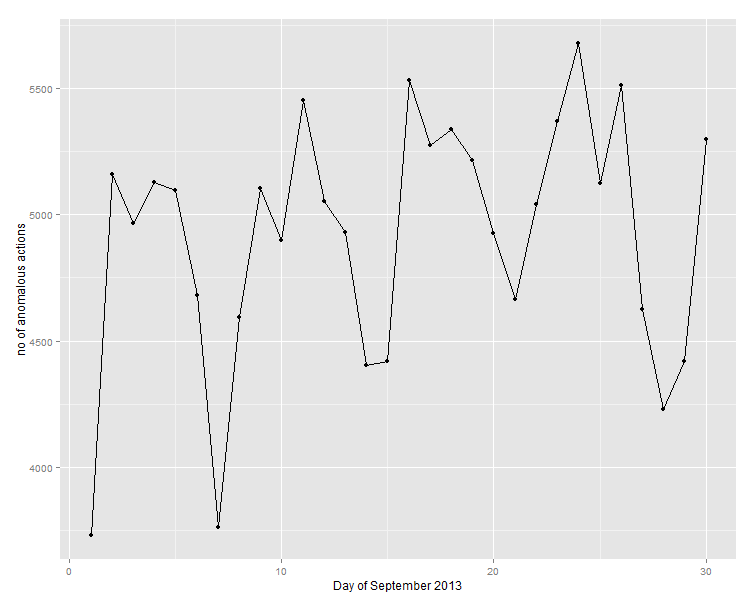 Well well… Now we really had something: our phantom was indeed a solitary one, it was present each and every day during September 2013, every time with abnormally, ridiculously high number of actions (in the order of thousands).
The phantom number of actions looked indeed abnormally high but, in fact, we didn’t know yet what a “normal” daily number of actions was. To do so, we had to add some lines in the script above, so as to calculate the average daily number of actions per registered user; and, since the comparison to the average might not be exactly “fair”, we wanted to also calculate the average number of actions only of the “top-5” most active users (per day). These calculations were performed for the remaining registered users, after we had removed the phantom one. To calculate these quantities, simply modify the script given above as follows:
# add this before the for loop:
ave.all <- ave.high <- rep(0, length(loglist))
# and these inside the for loop
df.true <- df.registered[RegisteredUserId %in% users[,id]]  # true registered users (anomalous removed)
ave.all[k] <- df.true[,.N, by=RegisteredUserId] %>% .[,N] %>% mean  # mean no of actions for all non-anomalous registered users
ave.high[k] <- df.true[,.N, by=RegisteredUserId] %>% .[,N] %>% sort(., decreasing=TRUE) %>% head(5) %>% mean # mean no of actions for top-5 (after sorting)
Now, let’s see how it looks like:
> library(ggplot2)
> toPlot <- data.frame(anom, ave.all, ave.high)
> ggplot(toPlot, aes(x=seq(1,nrow(toPlot)), y = value, color = variable)) +
+   geom_line(aes(y = anom, col = "phantom")) +
+   geom_line(aes(y = ave.all, col = "average (phantom removed)")) +
+   geom_line(aes(y = ave.high, col = "top-5 average (phantom removed)")) +
+   xlab('Day of September 2013') +
+   ylab('no of actions (registered users)')
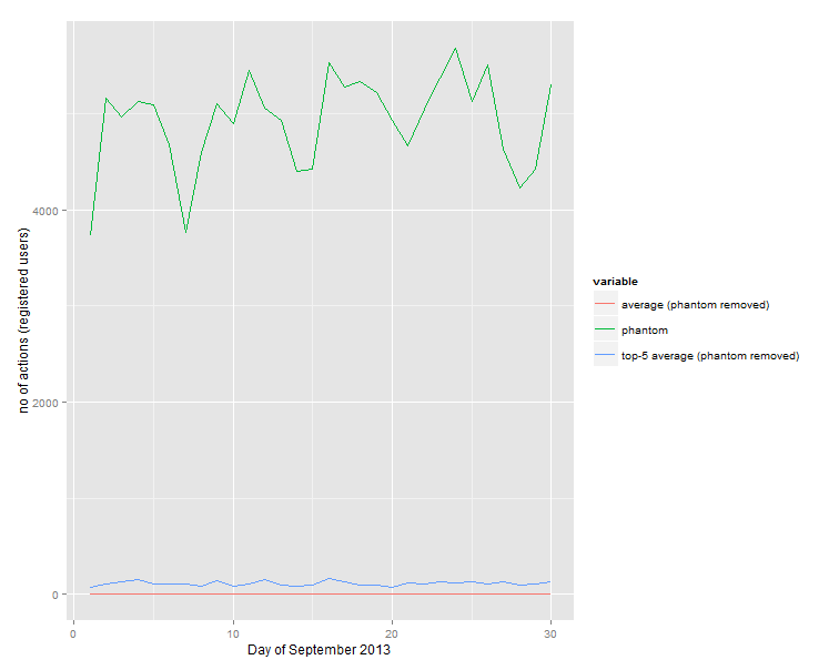
Judging from the plot above, the “abnormally high” characterization seems well-justified. And, since we cannot get an idea of the real average values due to the scale of the graph, let’s have a look at the actual numbers:
> toPlot
   anom  ave.all ave.high
1  3731 5.773129     71.4
2  5160 6.232456    106.8
3  4965 6.150500    134.2
4  5129 6.124104    151.0
5  5096 6.258704    109.8
6  4681 6.395717    104.0
7  3763 6.303743    103.2
8  4593 5.920359     83.2
9  5106 6.207052    135.8
10 4900 5.808309     85.0
11 5455 6.176329    106.4
12 5052 6.438385    155.8
13 4932 5.685059     89.2
14 4404 5.878244     82.0
15 4418 5.802864     95.6
16 5534 6.445458    159.4
17 5274 6.183803    128.4
18 5338 5.917961     96.6
19 5217 5.872186     96.0
20 4925 5.730159     69.8
21 4664 6.156940    118.4
22 5043 5.834975    101.4
23 5370 6.226553    126.0
24 5678 6.065283    121.2
25 5125 5.901831    134.0
26 5511 6.149225    107.2
27 4627 6.429160    130.2
28 4229 6.043307     97.2
29 4421 5.775728    102.8
30 5297 6.057870    128.2
So the number of the phantom actions on a daily basis was 3 orders of magnitude higher than the average of registered users, and 1-2 orders of magnitude higher than the average of the “top-5” most active (registered) users.
What exactly was it doing?
If you are working on a powerful machine with enough memory, like mine, you can actually load all log data in memory. The following script was used in order to sequentially read all the log files, merge them, and then save the resulting dataframe in a (3.1 GB) CSV file:
library(data.table)
setwd("C:/datathon/dataset")
f = '2013_09_01.log'
df = fread(f, header=FALSE)
names.df = c('sttp','UserSessionId', 'RegisteredUserId', 'PathURL',
             'action', 'Time', 'Query', 'CategoryId', 'ShopId',
             'ProductID', 'RefURL', 'SKU_Id','#Results')
setnames(df,names.df)
for (f in loglist[2:length(loglist)]) {
  temp = fread(f, header=FALSE)
  df <- rbind(df, temp, use.names=FALSE)
} # end for
rm(temp)
gc()
# export to single file:
write.csv(df, file='C:/datathon/dataset_full/all_logs.csv', row.names=FALSE, quote=TRUE)
We can now run some queries across the whole set of log data (30 days & about 13 million records):
> nrow(df)
[1] 13108692
> anoms <- df[RegisteredUserId == "cdc75a725963530a598e71c70677926b9a5f1bc1"] %>% nrow
> anoms
[1] 147638
> anoms/nrow(df) * 100
[1] 1.12626
So, it seems that our single phantom user was responsible for more that 1% of the whole traffic for September 2013 (that is, including all users – registered and unregistered)!
But what exact actions had it been performing?
The sttp attribute in the logs gives the type of request: 10, 22, or 800; in cases where sttp=800 (“user activity”), there is another attribute, action, that gives the specific type of the user activity request. Let’s check them:
> df[RegisteredUserId == "cdc75a725963530a598e71c70677926b9a5f1bc1"] %>% .[,.N, by=sttp]
   sttp      N
1:  800 147638
> df[RegisteredUserId == "cdc75a725963530a598e71c70677926b9a5f1bc1" & sttp == 800] %>% .[,.N, by=action]
   action      N
1:    csa 147638
As it turned out, for the whole month of September 2013 our phantom had been performing one and only one activity: csa (“add to comparison list”).
It is difficult to analyze the situation further without specific knowledge regarding the site and the possible activities; it is also well beyond the scope of this post. But before closing, I would like to offer a possible hint, following up to informal discussions with some datathon mentors and a judge during coffee breaks: we were told that such a behavior from a registered user was somewhat puzzling, especially regarding why such a user would bother to register; if I understood correctly, being a registered user does not imply any significant additional ‘privileges’ in the site.
But, at least according to the logs provided for the datathon, it turns out that non-registered users cannot perform 800-type activities:
> df[RegisteredUserId == ''] %>% .[,.N, by=sttp]
   sttp       N
1:   22 4223346
2:   10 8319379
So, given the specific type of activity our phantom had been performing in the site, we have at least a rational hint as to why it bothered to register, instead of just posing as an unregistered user (and hence leaving practically no trails at all).
“OK OK, you have convinced me – you have indeed found an anomaly! But why raising issues of data quality in your post title?”
Before explaining further, let me state the issue explicitly:
Anomaly detection always (and I mean ALWAYS) goes hand in hand with data quality.
Why am I stressing this? Because, as it became evident during the presentations, no other team had detected our phantom user! And everyone just went along to report that the percentage of actions by registered users in the logs was 4% (with at least one team reporting 5%).
Let’s see the actual and reported values (remember that now df holds the whole logs, i.e. about 13 million records):
> ratio.naive <- nrow(df[RegisteredUserId != ''])/nrow(df) * 100 > ratio.naive
[1] 4.317494
> anoms <- df[RegisteredUserId == "cdc75a725963530a598e71c70677926b9a5f1bc1"] %>% nrow
> reg <- df[RegisteredUserId != ''] %>% nrow - anoms # subtract anomalous from registered
> ratio.true <- reg/(nrow(df) - anoms) * 100 # and from the whole (denominator) > ratio.true
[1] 3.227585
> abs(ratio.naive - ratio.true)/ratio.true * 100
[1] 33.76857
The quantity ratio.naive above is 4.32%, for which the reported 4% is indeed a fair approximation (at least for a powerpoint “business” presentation). However, it should be clear by now that anomalies like the one represented by our phantom (registered) user should be removed from the data before calculating such quantities, since they do not represent “legitimate” registered users; if we do so, the true ratio becomes 3.23% (which would become simply 3% in a slide), and the reported value relative to the true one comes off by 34% (which may or may not be of business value, depending on the context, but certainly does not exactly count as a success).
Remember the datathon mentor quoted above, reminding us that “such issues in the data is something you are expected to deal with“?
Well, as I already said, I couldn’t agree more…
Wrapping up
To summarize: during the Athens Datathon 2015, we (i.e. me and Georgios Kaiafas) located a user in the provided log files, which was anomalous in at least three ways:
- He/she performed an extremely high number of actions, each and every day, for the whole month
- Although registered, he/she was not included in the registered users file
- All his/her actions were exclusively of one specific type
Moreover:
- We were the only team that located the anomaly
- It seemed that even the data provider was not aware of this phantom user
- Our finding invalidated certain quantities reported by almost all other teams
As I said in the introduction, I am writing this post mainly trying to share how an exploratory data analysis is performed, in practice and as-it-happens. So, let me try to distill some principles we followed, which I hope will be valuable to others:
- Always perform sanity checks!
- Regarding your sanity checks: don’t be lazy.
- Do not lightheartedly attribute your sanity check discrepancies to the “usual suspects” (which usually, and most conveniently, will be “somebody else’s fault”).
- Be alerted, and always ready to change course if necessary, depending on your findings.
- Follow your findings to the end – you may be surprised with what lies at the bottom of the rabbit’s hole.
- If you find an anomaly, check whether it may affect your data quality before proceeding to report aggregated results or even simple summary statistics.
* * *
Participating to the datathon was fun, really fun – OK, not exactly like competing in Kaggle, or patrolling with the UN in Western Sahara, but it came close enough… Many thanks to the organizers, the sponsors, and all the people who helped.
And it was a busy week, this last one: apart from the datathon, we also had the kick-off event of the Athens Data Science & Machine Learning meetup (which was very interesting indeed). Add to all these the newly formed AthensR group, and… well, I really hope we will get busier and busier with such events in the future…
* * *
Working along with Georgios Kaiafas was a sheer pleasure: I was already positively preoccupied, of course, but the reality proved to be even better – thanx mate!
> sessionInfo()
R version 3.1.2 (2014-10-31)
Platform: x86_64-w64-mingw32/x64 (64-bit)

locale:
[1] LC_COLLATE=English_United Kingdom.1252  LC_CTYPE=English_United Kingdom.1252    LC_MONETARY=English_United Kingdom.1252
[4] LC_NUMERIC=C                            LC_TIME=English_United Kingdom.1252

attached base packages:
[1] stats     graphics  grDevices utils     datasets  methods   base

other attached packages:
[1] ggplot2_1.0.1    magrittr_1.5     data.table_1.9.4

loaded via a namespace (and not attached):
 [1] chron_2.3-47     colorspace_1.2-6 digest_0.6.8     grid_3.1.2       gtable_0.1.2     MASS_7.3-35      munsell_0.4.2
 [8] plyr_1.8.3       proto_0.3-10     Rcpp_0.11.6      reshape2_1.4.1   scales_0.2.5     stringi_0.5-5    stringr_1.0.0
[15] tools_3.1.2

- Streaming data from Raspberry Pi to Oracle NoSQL via Node-RED - February 13, 2017
- Dynamically switch Keras backend in Jupyter notebooks - January 10, 2017
- sparklyr: a test drive on YARN - November 7, 2016
Could you please post the already anonymised data? It will help a lot trying to reproduce your results.
This would be ideal, but unfortunately I cannot do it myself; there was a clear understanding that, although of course we can write and blog about the event and the data, we cannot re-distribute the dataset ourselves (i.e. datathon participants). Only the data provider can do that (pinging them might not be a bad idea).
Iraklis, I am so glad collaborating with you and reveal such an surprising finding. In a few days I will send you the Python (Pandas) code and I think, it would be great to test execution time between our favorite tools.
Thanks, the pleasure was mine! Looking forward for the pandas code, although I think the data.table package will be proved way faster… 😉
And here’s a part of the follow-up conversation @Twitter:
[…] a previous post, we described how we performed exploratory data analysis (EDA) in real-world log files, as provided […]
[…] known as Oracle R Advanced Analytics for Hadoop – ORAAH). We will use the weblog data from Athens Datathon 2015, which we have already loaded in a Hive table named weblogs, as described in more detail in our […]
[…] us remind here that the weblogs data come from a use case which we have described in a previous post; to present an equivalent in-database analysis using ORE, we also create a regular (i.e. […]