Nonlinear regression using Spark – Part 2: sum-of-squares objective functions

This post is the second one in a series that discusses algorithmic and implementation issues about nonlinear regression using Spark. In the previous post we identified a small window for contribution into Spark MLlib by adding methods for nonlinear regression, starting with the definition and implementation of a general nonlinear model. We remind the reader that regression is essentially an optimization task that minimizes a sum-of-squares function. The boldface items in the list below indicate where we stand within the general picture of these series of posts:

1. Extend the linear model to a generic nonlinear one and provide practical examples of general models
2. Given a model and its derivatives, define an objective function and provide a novel way to calculate first and second order derivatives for all training data. This is based on the paper of Wilamowski and Yu, Improved Computation for Levenberg–Marquardt Training (IEEE Transactions on Neural Networks vol. 21, No. 6, June 2010).
3. Implement a Gauss-Newton optimization algorithm with line search, which is more robust than stochastic gradient descend (SGD) while still sharing the same distributed behavior (map-reduce). We also argue that our proposed Gauss-Newton implementation performs marginally better than the Limited-memory BFGS (L-BFGS) included in the Scala Breeze library.
4. Apply the above regression analysis to machine learning problems

Using the nonlinear model defined in the previous post, we will define a sum-of-squares objective function and exploit its special structure to calculate its derivatives. We will provide a distributed implementation using Spark RDDs, as well as a serial one using Breeze dense matrices and vectors. The calculated derivatives will be used in the optimization process.

Objective function

In the previous post we defined the NonlinearModel trait, along with two concrete implementations, namely  NeuralNetworkModel and GaussianMixtureModel.
Now that the model function is defined, we can proceed in implementing the objective function on which we are going to optimize (train) using a specific input dataset . We will use the term SumOfSquaresFunction as it reflects exactly the form of the function we minimize, i.e. it is essentially a sum of squared quantities iterated over the training set. This special form of the objective function is crucial for the analysis and implementation of the optimization algorithm, since we can exploit it to calculate second order derivatives. Recall that:

To see why the special form of the objective function often makes sum-of-squares problems easier to solve than general unconstrained minimization problems, we combine the individual components into a single residual vector as follows:

(1)  

Using this notation, we can rewrite as . The derivatives of can be expressed in terms of the Jacobian , which is the matrix of first partial derivatives of the residuals:

(2)  

where is the gradient of with respect to :

(3)  

The rightmost vector of Eq.(3) above contains the partial derivatives of the model function for a specific input vector. The analysis from this point onwards assumes that we can calculate these derivatives and we no longer care about specific nonlinear models.
The gradient and the Hessian (second order derivatives matrix) of can be expressed in matrix form as follows:

(4)  

The first partial derivatives of the residuals, and hence the Jacobian matrix , are relatively easy or inexpensive to calculate either analytically or numerically. We can thus obtain the gradient . Using , we can also calculate the first term in the Hessian matrix without evaluating any second derivatives of the functions . This is a distinctive feature of the sum-of-squares problems: the first part of the Hessian matrix can be computed using first order derivatives only. Moreover, this term is often more important than the second summation term in Eq.(4), because the residuals are either close to affine near the solution (that is, the are relatively small) or are themselves relatively small.

Most algorithms for nonlinear sum-of-squares exploit these structural properties of the Hessian and use the following approximation:

(5)  

We define a trait SumOfSquaresFunction to describe the basic methods exposed by the objective function. This trait extends Breeze trait DiffFunction[BDV[Double]], so that we can use the methods defined there. The methods exposed are:

1. def calculate(w: BDV[Double]): (Double, BDV[Double]): Given a set of tunable parameters, this method returns the objective function value and the gradient vector .
2. def hessian(w: BDV[Double]): BDM[Double]: Given a set of tunable parameters, this method returns a positive definite approximation of the Hessian matrix ().
3. getDim():Int: Returns the dimensionality of the objective function (equals the number of parameters of the underlying model).

import breeze.linalg.{DenseVector => BDV}
import breeze.linalg.{DenseMatrix => BDM}
import breeze.optimize.DiffFunction
import breeze.linalg._
/**
 * @author Nodalpoint
 */
trait SumOfSquaresFunction extends  DiffFunction[BDV[Double]] {
  def getDim():Int
  def calculate(weights: BDV[Double]): (Double, BDV[Double])
  def hessian(weights: BDV[Double]): BDM[Double]  
}

As we said in the introduction, in this series of posts we will implement two versions of the objective function: one suitable for large scale problems that uses distributed Spark RDDs and aggregate operations, and a second one for low/medium scale problems that will operate on Breeze dense vectors/matrices. As expected, both implementations are equivalent for low/medium scale problems, as we are going to demonstrate at the last section of this post.

Objective function implementation using Spark RDDs

One of the innovative ideas in this presentation is how to use RDD transformations and actions to perform in parallel all necessary function and derivative calculations for the sum-of-squares objective function. Some interesting ideas were presented by Wilamowski and Yu in Improved Computation for Levenberg–Marquardt Training (IEEE Transactions on Neural Networks vol. 21, No. 6, June 2010). In this paper, the authors propose a derivative calculation methodology for the case of sum-of-square functions with a large number of training instances. Recall the derivative equations for the case of sum-of-square functions:

(6)  

The common way to calculate Eq. (6) is first to calculate the complete Jacobian (iterate over the entire training set) and then perform summation along (the dimensionality of ). The idea of Wilamowski and Yu is to partially calculate the Jacobian on a per pattern basis, i.e. for each training pattern we calculate a column of the Jacobian and distributively aggregate the final outcome by addition. That way, we can implement a data parallel strategy for derivative calculation which is tailored to Spark!

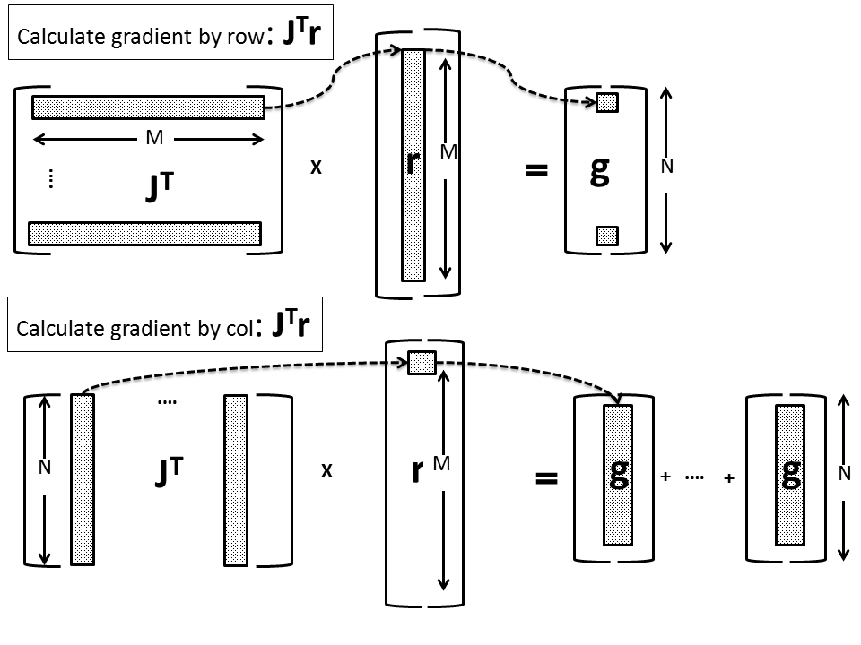
For the case of first order derivatives , instead of using the columns of the Jacobian matrix as dictated by Eq. (6) and calculate the gradient vector element by element, we can multiply the i-th Jacobian row with the i-th element of the residual vector and aggregate by addition the resulting vectors. This is shown schematically in the figure below (the bottom figure represents our implementation):

For the case of second order derivative, Wilamowski and Yu proposed a multiplication based on individual rows of the Jacobian matrix that leads to vectors and matrices. Normal multiplication would require all rows of Jacobian matrix to be calculated; with the new proposed scheme, we only require one row at a time. The partial results (vectors and matrices) are then aggregated by addition to form the final gradient vector or Hessian approximation. This is schematically displayed in the figure below (again, the bottom figure represents our implementation):

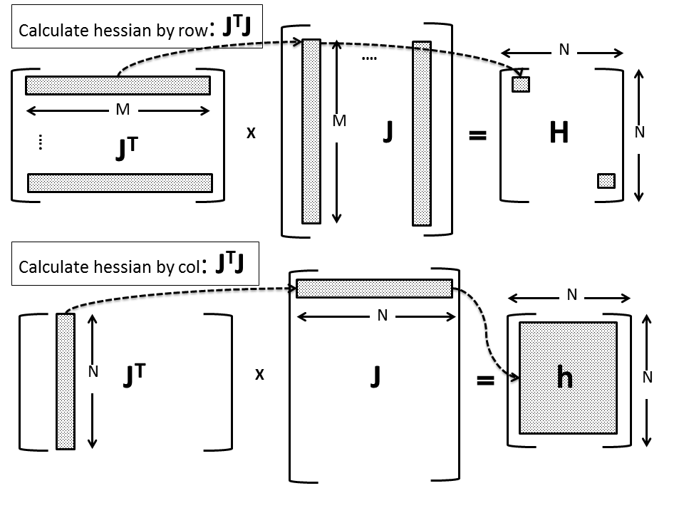
According to Wilamowski and Yu, a series of , subgradients and , subhessians are calculated per input pattern and aggregated over all training samples to produce the final outcome. The Spark implementation of stochastic gradient descent uses the same strategy implemented by the efficient treeAggregate() action. Our implementation presented here is a direct extension of this aggregation strategy to the calculation of the Hessian matrix approximation.

We are now ready to dive into the implementation details concerning Spark RDDs. Training data must provided in (input, output) pairs as RDD[(Vector, Double)]

import org.apache.spark.rdd._
import breeze.linalg.{DenseVector => BDV}
import breeze.linalg.{DenseMatrix => BDM}
import breeze.optimize.DiffFunction
import breeze.linalg._
import breeze.optimize.DiffFunction
import org.apache.spark.mllib.linalg.Vectors
import org.apache.spark.mllib.linalg.DenseVector
import org.apache.spark.mllib.linalg.DenseMatrix
import org.apache.spark.mllib.linalg.Vector
import org.apache.spark.mllib.linalg.Matrices
 
/**
 * @author Nodalpoint
 * Implementation of the sum-of-squares objective function using Spark RDDs
 * 
 *  Properties
 *    model: NonlinearModel -> The nonlinear model that defines the function
 *    data: RDD[(Double, Vector)] -> The training data used to calculate the loss in a form of a Spark RDD
 *                         that contains target, input pairs.
 *                         [(t1, x1), (t2, x2), ..., (tm, xm)]
 */
class SumOfSquaresFunctionRDD(fitmodel: NonlinearModel, xydata:RDD[(Double, Vector)]) extends  SumOfSquaresFunction {
  var model:NonlinearModel = fitmodel
  var dim = fitmodel.getDim()
  var data:RDD[(Double, Vector)] = xydata
  var m:Int = data.cache().count().toInt
  var n:Int = data.first()._2.size
  
/**
 * Return the objective function dimensionality which is essentially the model's dimensionality  
 */
def getDim():Int = {
    return this.dim
}
/**
 * This method is inherited by Breeze DiffFunction. Given an input vector of weights it returns the 
 * objective function and the first order derivative.
 * It operates using treeAggregate action on the training pair data.
 * It is essentially the same implementation as the one used for the Stochastic Gradient Descent
 * Partial subderivative vectors are calculated in the map step 
 *    val per = fitModel.eval(w, feat)  
      val gper = fitModel.grad(w, feat)
 * and are aggregated by summation in the reduce part.
 */
def calculate(weights: BDV[Double]): (Double, BDV[Double]) = {
  assert(dim == weights.length)
  val bcW = data.context.broadcast(weights)

  val fitModel:NonlinearModel = model
  val n:Int = dim
  val bcDim = data.context.broadcast(dim)

  val (grad, f) = data.treeAggregate((Vectors.zeros(n), 0.0))(
    seqOp = (c, v) => (c, v) match { case ((grad, loss), (label, features)) =>
      //fitModel.setWeights(bcW.value)
      val feat:BDV[Double] = new BDV[Double](features.toArray)
      val w:BDV[Double] = new BDV[Double](bcW.value.toArray)
      val per = fitModel.eval(w, feat)  
      val gper = fitModel.grad(w, feat)
      var f1 = 0.5*Math.pow(label-per, 2)
      var g1 = 2.0*(per-label)*gper
      
      val gradBDV = new BDV[Double](grad.toArray)
      var newgrad = Vectors.dense( (g1 + gradBDV).toArray)
  
    (newgrad, loss + f1)
     },
    combOp = (c1, c2) => (c1, c2) match { case ((grad1, loss1), (grad2, loss2)) =>
      //axpy(1.0, grad2, grad1)
      val grad1BDV = new BDV[Double](grad1.toArray)
      val grad2BDV = new BDV[Double](grad2.toArray)
      var newgrad = Vectors.dense( (grad1BDV+grad2BDV).toArray)
    (newgrad, loss1 + loss2)
   })

    val gradBDV = new BDV[Double](grad.toArray)
  return (f, gradBDV)
}
/**
 * This method calculates the Hessian matrix approximation using Jacobian matrix and
 * the algorithm of Wilamowsky and Yu.
 * It operates using treeAggregate action on the training pair data.
 * Partial subhessian matrices are calculated in the map step
 *    val gper = fitModel.grad(w, feat)
      val hper : BDM[Double] = (gper * gper.t)
 *  and aggregated by summation in the reduce part.
 * Extra care is taken to transform between Breee and Spark DenseVectors.
 */
def hessian(weights: BDV[Double]): BDM[Double] = {
  val bcW = data.context.broadcast(weights)

   val fitModel:NonlinearModel = model
   val n:Int = dim
   val bcDim = data.context.broadcast(dim)

    val (hess) = data.treeAggregate((new DenseMatrix(n, n, new Array[Double](n*n))))(
          seqOp = (c, v) => (c, v) match { case ((hess), (label, features)) =>
          val w:BDV[Double] = new BDV[Double](bcW.value.toArray)
          val feat:BDV[Double] = new BDV[Double](features.toArray)
          val gper = fitModel.grad(w, feat)
          val hper : BDM[Double] = (gper * gper.t)
          val hperDM:DenseMatrix = new DenseMatrix(n, n, hper.toArray ) 
  
          for (i<-0 until n*n){ hess.values(i)=hperDM.values(i)+hess.values(i) } (hess) }, combOp = (c1, c2) => (c1, c2) match { case ((hess1), (hess2)) =>
             for (i<-0 until n*n){
                hess1.values(i)=hess1.values(i)+hess2.values(i)
              }
          (hess1)
          })
          
          var hessBDM: BDM[Double] = new BDM[Double](n, n, hess.toArray)
          var Hpos = posDef(hessBDM)

          return Hpos
}


/**
 * Helper method that uses eigenvalue decomposition to enforce positive definiteness of the Hessian
 */
def posDef(H:BDM[Double]):BDM[Double] = {
    var n = H.rows
    var m = H.cols
    var dim = model.getDim()
    var Hpos :BDM[Double] = BDM.zeros(n, m)

    var eigens = eigSym(H)
    var oni:BDV[Double] = BDV.ones[Double](dim)
    var diag = eigens.eigenvalues
    var vectors = eigens.eigenvectors


    //diag = diag :+ (1.0e-4)
     for (i<-0 until dim){
        if (diag(i) < 1.0e-4){
          diag(i) = 1.0e-4
        }
    
      }


    var I = BDM.eye[Double](dim)
    for (i<-0 until dim){
      I(i, i) = diag(i)
    }

    Hpos = vectors*I*(vectors.t)
    return Hpos
  }    
}

Objective function implementation using Breeze

In the case of small- to medium-sized problems, we provide an implementation that stores data in Breeze DenseArrays and uses the full Jacobian matrix to calculate derivatives. This implementation can be also used to crosscheck the results of the RDD implementation – the results of both must match within the accuracy of double precision ().

import breeze.linalg.{DenseVector => BDV}
import breeze.linalg.{DenseMatrix => BDM}
import breeze.optimize.DiffFunction
import breeze.linalg._


/**
 * @author Nodalpoint
 * Implementation of the sum-of-squares objective function for small-sized problems where training data can fit in a
 * Breeze matrix. 
 * 
 *  Properties
 *    model: NonlinearModel -> The nonlinear model that defines the function
 *    data: DenseMatrix -> The training data used to calculate the loss in a form of a Breeze DenseMatrix
 *                         The first n columns are the input data and the n+1 column the target value
 */
class SumOfSquaresFunctionBreeze(fitmodel: NonlinearModel, xydata:BDM[Double]) extends  SumOfSquaresFunction{
  var model:NonlinearModel = fitmodel
  var dim = fitmodel.getDim()
  var data:BDM[Double] = xydata
  
  var m:Int = data.rows
  var n:Int = data.cols-1
  var Y:BDV[Double] = data(::, n)
  var X:BDM[Double] = data(::, 0 to n-1)

/**
 * Return the objective function dimensionality which is essentially the model's dimensionality  
 */
def getDim():Int = {
    return this.dim
}

/**
 * This method is inherited by Breeze DiffFunction. Given an input vector of weights it returns the 
 * objective function and the first order derivative
 */
def calculate(weights: BDV[Double]): (Double, BDV[Double]) = {
  assert(dim == weights.length)
  var f:Double = 0
  var grad:BDV[Double] = BDV.zeros(dim)
  
  var r:BDV[Double] = subsum(weights)
  f = 0.5 * (r.t * r)
  grad = granal(weights)

  return (f, grad)
}

/**
 * This method returns a positive definite approximation of the Hessian matrix at point w 
 */
def hessian(weights: BDV[Double]): BDM[Double] = {
   var H = hanal(weights)
   
   var Hpos = posDef(H)
   return Hpos
}

/**
 * Helper method that returns a vector of errors per training input.
 * It uses model.eval() for each input 
 */
def subsum(weights: BDV[Double]):BDV[Double] = {
    var f:BDV[Double] = BDV.zeros(m)
    var per:Double = 0

    for (i <- 0 to m-1){
      var x: BDV[Double] = X(i, ::).t
      per = model.eval(weights, x)  
      f(i) = per - Y(i)
    }
    return f
}

/**
 * Helper method that returns the gradient of the objective function after 
 * iterating through whole the training set
 */
def granal(weights: BDV[Double]): BDV[Double] = {
   var g:BDV[Double] = BDV.zeros(dim)
   var gper:BDV[Double] = BDV.zeros(dim)
   var ff:BDV[Double] = subsum(weights)

   for (i<-0 to m-1){
     var x: BDV[Double] = X(i, ::).t
     gper = model.grad(weights, x)
     for (j<-0 to dim-1){
        g(j) = g(j) + 2.0*ff(i)*gper(j) 
     }
   }
   return g
}

/**
 * Helper method that returns the Jacobian matrix. Partial derivative of j-th pattern and i-th input 
 */
def janal(weights: BDV[Double]):BDM[Double] = {
  var J:BDM[Double] = BDM.zeros(m, dim)
  var gper:BDV[Double] = BDV.zeros(dim)

  for (i<-0 to m-1){
    var x: BDV[Double] = X(i, ::).t
    gper = model.grad(weights, x)
    for (j <- 0 to dim-1){
      J(i, j) = gper(j)             
    }
  }

  return J
}

/**
 * Helper method that returns the Hessian matrix approximation using the Jacobian
 */
def hanal(weights: BDV[Double]):BDM[Double] = {
  var J = janal(weights)

   return J.t * J
}

/**
 * Helper method that uses eigenvalue decomposition to enforce positive definiteness of the Hessian
 */
def posDef(H:BDM[Double]):BDM[Double] = {
    var n = H.rows
    var m = H.cols
    var dim = model.getDim()
    var Hpos :BDM[Double] = BDM.zeros(n, m)

    var eigens = eigSym(H)
    var oni:BDV[Double] = BDV.ones[Double](dim)
    var diag = eigens.eigenvalues
    var vectors = eigens.eigenvectors


   // diag = diag :+ (1.0e-4)
    for (i<-0 until dim){
        if (diag(i) < 1.0e-4){
          diag(i) = 1.0e-4
        }
    }

    var I = BDM.eye[Double](dim)
    for (i<-0 until dim){
      I(i, i) = diag(i)
    }

    Hpos = vectors*I*(vectors.t)
    return Hpos
  }    
}

Testing the objective function implementation

In this section, we provide a simple application to test the implementation of the sum-of-squares objective function. First we created some test training data that map a two dimensional input to a target value. This training set was created artificially for demonstration purposes and corresponds to a saddle-like 2D function shown in the figure below:

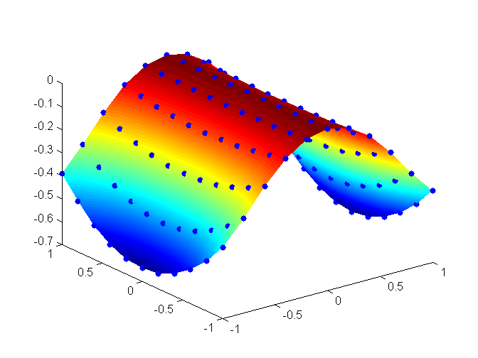
For completeness we provide the data set in triplets:

-1.000000,-1.000000,-0.389030
-1.000000,-0.800000,-0.479909
-1.000000,-0.600000,-0.550592
-1.000000,-0.400000,-0.601080
-1.000000,-0.200000,-0.631373
-1.000000,0.000000,-0.641471
-1.000000,0.200000,-0.631373
-1.000000,0.400000,-0.601080
-1.000000,0.600000,-0.550592
-1.000000,0.800000,-0.479909
-1.000000,1.000000,-0.389030
-0.800000,-1.000000,-0.290037
-0.800000,-0.800000,-0.354534
-0.800000,-0.600000,-0.404698
-0.800000,-0.400000,-0.440530
-0.800000,-0.200000,-0.462029
-0.800000,0.000000,-0.469195
-0.800000,0.200000,-0.462029
-0.800000,0.400000,-0.440530
-0.800000,0.600000,-0.404698
-0.800000,0.800000,-0.354534
-0.800000,1.000000,-0.290037
-0.600000,-1.000000,-0.174592
-0.600000,-0.800000,-0.212638
-0.600000,-0.600000,-0.242229
-0.600000,-0.400000,-0.263365
-0.600000,-0.200000,-0.276047
-0.600000,0.000000,-0.280274
-0.600000,0.200000,-0.276047
-0.600000,0.400000,-0.263365
-0.600000,0.600000,-0.242229
-0.600000,0.800000,-0.212638
-0.600000,1.000000,-0.174592
-0.400000,-1.000000,-0.079523
-0.400000,-0.800000,-0.096729
-0.400000,-0.600000,-0.110112
-0.400000,-0.400000,-0.119671
-0.400000,-0.200000,-0.125406
-0.400000,0.000000,-0.127318
-0.400000,0.200000,-0.125406
-0.400000,0.400000,-0.119671
-0.400000,0.600000,-0.110112
-0.400000,0.800000,-0.096729
-0.400000,1.000000,-0.079523
-0.200000,-1.000000,-0.019993
-0.200000,-0.800000,-0.024311
-0.200000,-0.600000,-0.027670
-0.200000,-0.400000,-0.030070
-0.200000,-0.200000,-0.031509
-0.200000,0.000000,-0.031989
-0.200000,0.200000,-0.031509
-0.200000,0.400000,-0.030070
-0.200000,0.600000,-0.027670
-0.200000,0.800000,-0.024311
-0.200000,1.000000,-0.019993
0.000000,-1.000000,0.000000
0.000000,-0.800000,0.000000
0.000000,-0.600000,0.000000
0.000000,-0.400000,0.000000
0.000000,-0.200000,0.000000
0.000000,0.000000,0.000000
0.000000,0.200000,0.000000
0.000000,0.400000,0.000000
0.000000,0.600000,0.000000
0.000000,0.800000,0.000000
0.000000,1.000000,0.000000
0.200000,-1.000000,-0.019993
0.200000,-0.800000,-0.024311
0.200000,-0.600000,-0.027670
0.200000,-0.400000,-0.030070
0.200000,-0.200000,-0.031509
0.200000,0.000000,-0.031989
0.200000,0.200000,-0.031509
0.200000,0.400000,-0.030070
0.200000,0.600000,-0.027670
0.200000,0.800000,-0.024311
0.200000,1.000000,-0.019993
0.400000,-1.000000,-0.079523
0.400000,-0.800000,-0.096729
0.400000,-0.600000,-0.110112
0.400000,-0.400000,-0.119671
0.400000,-0.200000,-0.125406
0.400000,0.000000,-0.127318
0.400000,0.200000,-0.125406
0.400000,0.400000,-0.119671
0.400000,0.600000,-0.110112
0.400000,0.800000,-0.096729
0.400000,1.000000,-0.079523
0.600000,-1.000000,-0.174592
0.600000,-0.800000,-0.212638
0.600000,-0.600000,-0.242229
0.600000,-0.400000,-0.263365
0.600000,-0.200000,-0.276047
0.600000,0.000000,-0.280274
0.600000,0.200000,-0.276047
0.600000,0.400000,-0.263365
0.600000,0.600000,-0.242229
0.600000,0.800000,-0.212638
0.600000,1.000000,-0.174592
0.800000,-1.000000,-0.290037
0.800000,-0.800000,-0.354534
0.800000,-0.600000,-0.404698
0.800000,-0.400000,-0.440530
0.800000,-0.200000,-0.462029
0.800000,0.000000,-0.469195
0.800000,0.200000,-0.462029
0.800000,0.400000,-0.440530
0.800000,0.600000,-0.404698
0.800000,0.800000,-0.354534
0.800000,1.000000,-0.290037
1.000000,-1.000000,-0.389030
1.000000,-0.800000,-0.479909
1.000000,-0.600000,-0.550592
1.000000,-0.400000,-0.601080
1.000000,-0.200000,-0.631373
1.000000,0.000000,-0.641471
1.000000,0.200000,-0.631373
1.000000,0.400000,-0.601080
1.000000,0.600000,-0.550592
1.000000,0.800000,-0.479909
1.000000,1.000000,-0.389030

The code of the sample application is shown below. We define an Object SumOfSquareTest that reads the training data and creates RDD and Breeze objective function implementations. The model used in this example is a Neural Network with two hidden nodes. It is left as a small exercise to the reader to change the model to a Gaussian Mixture Model with two nodes. The small change needed is given in one line below:

     var model: NonlinearModel = new GaussianMixtureModel(n, nodes)

import org.apache.spark.SparkContext
import org.apache.spark.SparkContext._
import org.apache.spark.SparkConf
import org.apache.spark.rdd._
import org.apache.spark.mllib.regression.LabeledPoint
import org.apache.spark.mllib.linalg.Vectors
import org.apache.spark.mllib.linalg.DenseVector
import org.apache.spark.mllib.linalg.Vector
import org.apache.log4j.Logger
import org.apache.log4j.Level
import breeze.linalg.{DenseVector => BDV}
import breeze.linalg._
import breeze.optimize.DiffFunction
import breeze.optimize.StrongWolfeLineSearch
import breeze.optimize.LineSearch
import org.apache.spark.rdd._
import org.apache.spark.mllib.linalg.Vectors
import org.apache.spark.mllib.linalg.DenseVector
import org.apache.spark.mllib.linalg.Vector
import breeze.io.CSVReader
import breeze.linalg.{DenseMatrix => BDM}
import breeze.stats.distributions._
import org.apache.commons.math3.random.{MersenneTwister, RandomGenerator}
import breeze.optimize.LBFGS
import breeze.optimize.MinimizingLineSearch

/**
 * @author Nodalpoint
 * A simple application to test the objective function implementation
 * Training data set:
 * <----- Input ----->  Target
 * -1.000000,-1.000000,-0.389030
 * -1.000000,-0.800000,-0.479909
 * -1.000000,-0.600000,-0.550592
 *  ...
 *  ...
 *  1.000000,1.000000,-0.389030
 */

object SumOfSquareTest {

	def main(args: Array[String]) = {
    /* Input dimension is 2*/
    var n:Int = 2
    /* Number of hidden nodes for the Neural Network */
    var nodes:Int = 4
    /* Read training data : Breeze style*/
    var XY: BDM[Double] = breeze.linalg.csvread(new java.io.File("/home/osboxes/workspace1/NonLinearRegression1/input.txt"))
    /* Number of training data*/
    var m:Int = XY.rows
    
    /*Create a neural network nonlinear model with input dimension 2 and 4 hidden nodes*/
    var model: NonlinearModel = new NeuralNetworkModel(n, nodes)
    /* The dimensionality of the tunable parameters */
    var dim: Int = model.getDim()
    /* A random vector containing some initial parameters for the model 
     * We are not optimizing in this demo */
    var w = BDV.rand[Double](dim)
    
    /*
     * Define a SumOfSquaresFunction based on Breeze using the neural network model  
     */
    var modelfunBreeze :SumOfSquaresFunction = new  SumOfSquaresFunctionBreeze(model, XY)
    /*
     * Calculate function value and derivatives at the initial random point w 
     */
    var (f, g) = modelfunBreeze.calculate(w)
    var H = modelfunBreeze.hessian(w)
    System.out.println("--- Neural Network Model (Breeze Implementation) ---")
    System.out.println("Weights w = " + w)
    System.out.println("Error function = " + f)
    System.out.println("Gradient (first 5 elements)  :")
    System.out.println( g )
    System.out.println("Hessian : ")
    System.out.println(H(0, ::))
    
    
    Logger.getLogger("org").setLevel(Level.OFF)
    Logger.getLogger("akka").setLevel(Level.OFF)
    val conf = new SparkConf().setAppName("Sample Application").setMaster("local[2]")
    val sc = new SparkContext(conf)
    /* Read training data : Spark style*/
    val dataTxt = sc.textFile("/home/osboxes/workspace1/NonLinearRegression1/input.txt", 2)
    /* Split the input data into target, input pairs (Double, Vector) */ 
    val data = dataTxt.map { 
        line =>
        val parts = line.split(',')
        (parts(parts.length-1).toDouble, Vectors.dense(parts.take(parts.length-1).map(_.toDouble)))
    }.cache() 
    /* Number of training data*/
    val numExamples = data.count()
    
     /*
     * Define a SumOfSquaresFunction based on RDDs using the neural network model  
     */   
    var modelfunRDD :SumOfSquaresFunction = new  SumOfSquaresFunctionRDD(model, data)
    /*
     * Calculate function value and derivatives at the initial random point w 
     */    
    var (f1, g1) = modelfunRDD.calculate(w)
    var H1 = modelfunRDD.hessian(w)
    System.out.println("--- Neural Network Model (RDD Implementation) ---")
    System.out.println("Weights w = " + w)
    System.out.println("Error function = " + f1)
    System.out.println("Gradient (first 5 elements)  :")
    System.out.println( g1)
    System.out.println("Hessian : ")
    System.out.println(H1(0, ::))
    
    /* 
     * Compare the two implementation results. They should be identical 
     * within the double precision accuracy
     */
    System.out.println("Diff f " + Math.abs(f-f1) )
    System.out.println("Diff g " + norm(g-g1) )
    System.out.println("Diff H row 0 " + norm(H(::, 0)-H1(::, 0)) )
    System.out.println("Diff H row 1 " + norm(H(::, 1)-H1(::, 1)) )
    System.out.println("Diff H row 2 " + norm(H(::, 2)-H1(::, 2)) )

  }
}

The output of the sample application shows that the two implementations (Spark & Breeze) are equivalent: for the same training set they produce identical results.

--- Neural Network Model (Breeze Implementation) ---
Weights w = DenseVector(0.4031406990832569, 0.9572383668529576, 0.5710130380373641, 0.7536948019588541, 0.34555576655869547, 0.183090479644201, 0.05291928964737003, 0.5552500033518635, 0.6586262647716032, 0.9122094102132212, 0.23461555552578095, 0.42329340982825303, 0.1609637244480735, 0.43813247176159376, 0.6833677130462232, 0.7375603886004336)
Error function = 184.6608616266911
Gradient (first 5 elements)  :
DenseVector(0.2902691078896141, -1.0399841269881147, 65.35006066083868, 269.160282197041, 2.359408927034523, 4.382619017475873, 56.6847645097874, 216.35615264065294, 0.4742907974378115, 1.4763086408392236, 38.500812471097184, 239.23631492010904, 1.6361555448362481, 1.6255067630787727, 66.44722266004034, 278.763788919762)
Hessian : 
Transpose(DenseVector(1.2716372637210196, -0.11508025393014325, -0.1877610514610355, 0.17062327128799362, 1.0469056542950164, -0.06910831405599742, -0.09740127761257177, 0.29533218278814893, 0.7210073263057541, -0.10125739375489587, -0.08623520887023511, 0.6949133528823834, 1.2695727176325062, -0.06982971055578695, -0.15990500893505794, -0.20992492108432428))

Using Spark's default log4j profile: org/apache/spark/log4j-defaults.properties
15/12/18 09:13:54 INFO Remoting: Starting remoting
15/12/18 09:13:55 INFO Remoting: Remoting started; listening on addresses :[akka.tcp://sparkDriver@10.0.2.15:60775]
[Stage 0:>                                                          (0 + 0) / 2]
[Stage 0:>                                                          (0 + 2) / 2]
 --- Neural Network Model (RDD Implementation) ---
Weights w = DenseVector(0.4031406990832569, 0.9572383668529576, 0.5710130380373641, 0.7536948019588541, 0.34555576655869547, 0.183090479644201, 0.05291928964737003, 0.5552500033518635, 0.6586262647716032, 0.9122094102132212, 0.23461555552578095, 0.42329340982825303, 0.1609637244480735, 0.43813247176159376, 0.6833677130462232, 0.7375603886004336)
Error function = 184.66086162669117
Gradient (first 5 elements)  :
DenseVector(0.2902691078896069, -1.0399841269881138, 65.3500606608387, 269.1602821970411, 2.3594089270345275, 4.382619017475872, 56.6847645097874, 216.3561526406528, 0.47429079743781344, 1.4763086408392243, 38.50081247109718, 239.236314920109, 1.636155544836246, 1.6255067630787727, 66.44722266004037, 278.76378891976196)
Hessian : 
Transpose(DenseVector(1.2716372637210256, -0.11508025393014393, -0.1877610514610369, 0.17062327128799498, 1.0469056542950217, -0.06910831405599854, -0.09740127761257245, 0.2953321827881442, 0.721007326305757, -0.10125739375489673, -0.08623520887023664, 0.6949133528823859, 1.269572717632512, -0.06982971055578845, -0.1599050089350596, -0.20992492108432648))

Diff f 8.526512829121202E-14
Diff g 1.957050340653598E-13
Diff H row 0 1.2301788074630057E-14
Diff H row 1 9.379875535232206E-15
Diff H row 2 6.744785483306968E-14

You can download the code from here. You can use the sbt utility to create an eclipse project like described in this post. Then import the project in eclipse and run the SumOfSquareTest.scala file as a Scala application. Before running the code, make sure that you provide the correct path to the input.txt file. In this demo we do not tune the model parameters.

Summary

In this post, we have defined a sum-of-squares objective function to be used for minimizing the error in nonlinear regression. The objective function contains a nonlinear model described here that defines its dimensionality. The special sum-of-squares form allows us to approximate second order derivatives using the Jacobian, and Spark RDDs operations allow this computation in a distributed column-by-column fashion.

This first and second order derivative computation using Spark RDDs (treeAggregate()) constitutes the main contribution of this post.

In the next post of this series, we will actually minimize the objective function (train or fit the nonlinear model) using the training data set. We will use Spark & Breeze optimization algorithms, and we are going to implement the Gauss-Newton optimization algorithm for sum-of-squares objective functions.

• Author
• Recent Posts

Constantinos Voglis

Constantinos Voglis is one of our resident Data Scientists. He holds a PhD in numerical optimization methods and he has numerous academic publications in the field, including its applications in machine learning and graph processing. He is currently working on machine learning algorithms that originate from big data analysis tasks.

Latest posts by Constantinos Voglis (see all)

• Nonlinear regression using Spark – Part 2: sum-of-squares objective functions - October 31, 2016
• How to evaluate R models in Azure Machine Learning Studio - August 24, 2016
• Nonlinear regression using Spark – Part 1: Nonlinear models - February 10, 2016