Regression constitutes a very important topic in supervised learning. Its goal is to predict the value of one or more continuous target variables  (responses) given the value of a
  -dimensional vector
  of input variables (predictors). More specifically, given a training data set comprising of
  observations
  , where
  , together with corresponding target values
  , the goal is to predict the value of
  for a new value of
  . In the simplest approach, this can be done by directly constructing an appropriate function
  , parametrized by
  , whose values for new inputs
  constitute the predictions for the corresponding values of
  . The key point in this approach is to calculate appropriate values for such that the function best matches for all
  .
.
In a series of posts starting with this one, we will address the problem of nonlinear regression using Spark, where is a nonlinear function on , and provide code that utilizes Spark RDDs to implement the data distribution. Up to the current version (1.6.0), Spark’s MLlib provides only linear models for regression (e.g. linear regression with L1, L2, and elastic-net regularization), i.e. the case where
![\[y\left(\mathbf{x^{(i)}}, \mathbf{w}\right) = \mathbf{w}^T \mathbf{x} = w_1 x^{(i)}_1 + w_2 x^{(i)}_2 + \cdots + w_d x^{(i)}_n\]](https://www.nodalpoint.com/wp-content/ql-cache/quicklatex.com-9e191da42a11039a0d0c558442c89c13_l3.png "Rendered by QuickLaTeX.com")
is a simple linear function on . Quoting from the MLlib programming guide “Behind the scene, MLlib implements a simple distributed version of stochastic gradient descent (SGD), building on the underlying gradient descent primitive“. Our contribution can be resumed in the following topics:
- Extend the linear model to a generic nonlinear one and provide practical examples of general models
- Given a model and its derivatives, define an objective function and provide a novel way to calculate first and second order derivatives for all training data.; this is based on the paper of Wilamowski and Yu, Improved Computation for Levenberg–Marquardt Training. We provide two implementations for the objective function: a distributed implementation based on RDDs for large training sets, and a serial one based on Breeze DenseMatrix for small and medium-sized problems.
- Implement a Gauss-Newton optimization algorithm with line search, which is more robust than SGD and still shares the same distributed behavior (map-reduce). We also argue that the provided Gauss-Newton implementation performs marginally better than the Limited-memory BFGS (L-BFGS) included in the Scala Breeze package.
- Apply the above optimization methods to machine learning problems (regression analysis).
The target audience for these series of posts can be
- Machine learning practitioners and Spark users who would like to extend their methodology and test a nonlinear model. There is also room for researchers to devise a stochastic version of the proposed algorithm, where not all training data are presented before each weight update.
- Optimization practitioners who would like to use and extend a Scala implementation of the Gauss-Newton algorithm.
- Distributed computing researchers that would like to study the scaling of the distributed computation for the derivatives.
Let’s start with some basic definitions. For all the equations in this article, boldface letters will be used to denote vectors. We denote by the dimensionality of  (the input), by the number of training pairs (observations) and
  the number of tunable weights. So
![\[\mathbf{x}^{(i)} = \left ( \begin{array}{c} x^{(i)}_1 \\ x^{(i)}_2 \\ \vdots \\ x^{(i)}_n \end{array} \right )\]](https://www.nodalpoint.com/wp-content/ql-cache/quicklatex.com-d407a4897ccaf49d1ad6324df31cb835_l3.png "Rendered by QuickLaTeX.com")
will denote the  th,
th,  dimensional training input (
 ),
),
![\[\mathbf{t} = \left ( \begin{array}{c} t^{(1)} \\ t^{(2)} \\ \vdots \\ t^{(M)} \end{array} \right )\]](https://www.nodalpoint.com/wp-content/ql-cache/quicklatex.com-8977f7b4ec0c759f7261e1a37a8424f2_l3.png "Rendered by QuickLaTeX.com")
will denote the vector of all training outputs, and
![\[\mathbf{w} = \left ( \begin{array}{c} w_1 \\ w_2 \\ \vdots \\ w_N \end{array} \right )\]](https://www.nodalpoint.com/wp-content/ql-cache/quicklatex.com-fec2c661b1a24e1e131f7cdbd4972478_l3.png "Rendered by QuickLaTeX.com")
will denote the  dimensional vector of weights. Notice that in the linear case
  , whereas in the more general nonlinear case this is not true.
Training – Fitting – Optimizing
Tuning the model’s parameters requires two things:
- A set of pairs
 . This is usually called the training set.
 - An error function that measures the “closeness” between and . A common choice is the square error
 .
.
It is common in practice to use k-fold cross-validation techniques in order to reduce the effect of a specific training set on the tuning process. That way the resulting parameters are less biased to the initial training test.
The process of modifying the model’s parameters using a training set and an error function is known by several names, depending on the context: in machine learning, it is usually called training; in statistics it is called fitting; in any case, it is essentially an optimization process, since we actually minimize an error (loss) function (possibly with constraints). Since here we are mainly interested for machine learning applications, in the rest of this post we will stick to the term “training”.
Formally, the training process over a training set  , can be presented as an optimization (minimization) problem of the following loss function:
![\[f(\mathbf{w}) = \frac{1}{2} \sum_{i=1}^{M} e_i \left (y\left(\mathbf{x}^{(i)},\mathbf{w}\right), t^{(i)} \right ), \ \ \in \mathrm{R}^N\]](https://www.nodalpoint.com/wp-content/ql-cache/quicklatex.com-52b49b2d0d934d33075e8eccd63977f2_l3.png "Rendered by QuickLaTeX.com")
For the square error case, the loss function can be written as:
![\[f(\mathbf{w}) = \frac{1}{2} \sum_{i=1}^{M} \left( y\left(\mathbf{x}^{(i)}, \mathbf{w}\right) - t^{(i)} \right )^2 , \ \ \in \mathrm{R}^N\]](https://www.nodalpoint.com/wp-content/ql-cache/quicklatex.com-0a2c079431af9e44e7a0e8889663c971_l3.png "Rendered by QuickLaTeX.com")
The objective function  in the case of nonlinear modeling is not convex, and it is expected to have multiple local and global minima. So what we gain in flexibility we loose in computational complexity of locating the best minimum. This must be realized by all machine learning and optimization practitioners that use nonlinear models. However, this optimization difficulty is compensated by the increased expressiveness of the model.
Nonlinear regression models
A nonlinear regression model is the realization of the function that takes as input an  dimensional vector of weights as well as an input vector . The regression model is controlled by its weights, and for a sophisticated algorithm to operate we need its derivatives with respect to them:
(1) 
We can begin our implementation in Scala (utilizing the Breeze library) by defining the abstract trait of a nonlinear model with the following methods:
eval(w, x): the model’s response for input for a predefined set of parameters grad(w, x): the model’s partial derivative with respect to for input . It returns an dimensional vector
getDim(): The number of the model’s tunable parameters ()
We also include a method gradnumer(w, x) that numericaly approximates the derivatives grad(w, x).
import breeze.linalg.{DenseVector => BDV}
import breeze.linalg._

/**
 * @author Nodalpoint
 * All models used in least squares fitting must implement methods from this
 * abstract class
 */

trait NonlinearModel{
  /*
   * Model's output for a single input instance t
   * y(x; w) for fixed set of weights w
   */
  def eval(w: BDV[Double], x: BDV[Double]): Double
   /*
   * Model's derivative for a single input instance t
   * d(y(x, w)) / dw
   */
  def grad(w: BDV[Double], x: BDV[Double]): BDV[Double]
  /*
   * Model's dimensionality
   */
  def getDim(): Int
  /*
   * Model's derivative for a single input instance t
   * d(y(x, w)) / dw calculated numerically using forward differences
   */
  def gradnumer(w: BDV[Double], x: BDV[Double]): BDV[Double]
}
Using this abstract and general definition of a NonlinearModel, we can define any complicated and nonlinear model. Extra care must be given to maintain a mapping between the vector and the specific model parameters. For performance reasons, the user is advised to calculate the derivatives of the model analytically; one only needs to calculate the derivatives of considering constant and differentiate along  . Once the output and the derivatives of the model are defined for a single input
  , the code we present in this post will automatically generalize the output and derivatives for the whole training test.
A neural network model
The first model function we implement is a feedforward single-layered neural network. The network is fully connected and consists of  tunable parameters (weights), where
  is the number of hidden nodes and is the size of the input. Each hidden layer node sums the weighted input from the input nodes plus the bias (1) and applies a sigmoid activation function. The neural network with 3 input nodes and 3 hidden nodes is schematically represented as follows:
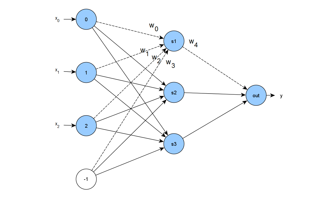
For each hidden layer node we define  weights: from the input,
  from the bias and to the output node. Thus in total we have
  tunable weights. If we use the numbering of weights suggested in the figure above, we can define a neural network model function algebraically as:
(2) 
where  is the output weight of hidden node ,
  is the bias weight for the hidden node , and
  are the weights from the input nodes. The neural network model is implemented in the class
 NeuralNetworkModel, shown below, that takes two constructor parameters: the input dimension and the size of hidden nodes . The class extends Serializable, since we want to execute it inside the closure of an RDD (more on this later); it also implements all methods of the trait NonlinearModel we have defined above.
import breeze.linalg.{DenseVector => BDV}
import breeze.linalg._

/**
 * @author Nodalpoint
 */
class NeuralNetworkModel(inputDim : Int, hiddenUnits:Int)
                                       extends Serializable  with NonlinearModel {
  var nodes: Int = hiddenUnits
  var n:Int = inputDim
  var dim:Int =  (n+2)*nodes

  def eval(w:BDV[Double], x: BDV[Double]) : Double = {
    assert(x.size == n)
    assert(w.size == dim)
    var f : Double = 0.0
    for (i <- 0 to nodes-1){
      var arg: Double  = 0.0
      for (j <- 0 to n-1){
         arg = arg + x(j)*w(i*(n+2)+j)
      }
      arg = arg + w(i*(n+2) + n)
      f = f + w(i*(n+2) + n + 1) / ( 1.0 + Math.exp(-arg))
    }
    return f
  }

  def grad(w:BDV[Double], x: BDV[Double]) : BDV[Double] = {
	  assert(x.size == n)
	  assert(w.size == dim)

	  var gper : BDV[Double] = BDV.zeros(dim) // (n+2)*nodes

	  for (i <- 0 to nodes-1){
		  var arg: Double  = 0
			for (j <- 0 to n-1){
			  arg = arg + x(j)*w(i*(n+2)+j)
			}
	                arg = arg + w(i*(n+2) + n)
			var sig : Double = 1.0 / ( 1.0 + Math.exp(-arg))

			gper(i*(n+2) + n + 1) = sig
			gper(i*(n+2) + n) =  w(i*(n+2) + n + 1)  * sig * (1-sig)
			for (j <- 0 to n-1){
				gper(i*(n+2)+j) = x(j) * w(i*(n+2) + n + 1)  * sig * (1-sig)
			}
	  }
	  return gper;
  }

  def getDim(): Int = {
  	return dim
  }

  def getNodes() :Int  = {
  	return nodes
  }

  def setNodes(n : Int)  = {
  	nodes = n
  	dim = (n+2) * nodes
  }

  def gradnumer(w:BDV[Double], x: BDV[Double]) : BDV[Double] = {
  	var h: Double = 0.000001
  	var g:BDV[Double] = BDV.zeros(this.dim)
  	var xtemp:BDV[Double] = BDV.zeros(this.dim)
  	xtemp = w.copy
  	var f0 = eval(xtemp, x)

  	for (i<-0 until this.dim){
  	        xtemp = w.copy
  		xtemp(i) += h
  		var f1 = eval(xtemp, x)
  		g(i) = (f1-f0)/h
  	}
  	return g
  }
}
A Gaussian mixture model
A Gaussian mixture model is a sum of  multivariate Gaussian functions of the form:
(3) 
where  is a scaling parameter,
  is the center of the distribution, and the covariance matrix
  is positive definite. In the figure below we present three surface plots of 2D Gaussians centered at
 ![[0, 0]^T](https://www.nodalpoint.com/wp-content/ql-cache/quicklatex.com-37683e38c4fc97040ca58f0143cf7c08_l3.png "Rendered by QuickLaTeX.com") . Each plot was generated using a different structure for the covariance matrix
. Each plot was generated using a different structure for the covariance matrix  . In the first symmetric case
  is a diagonal matrix will all elements equal.
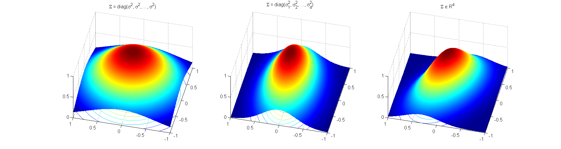
The second case represents a diagonal covariance matrix with different entries in the diagonal, that is slightly elongated in one dimension. Finally, the third case shown above is the general one, where the non-diagonal elements of the covariance matrix define rotation of the shape. For our demonstration here, we implement the second case, where we need only the parameters  in the diagonal of the covariance matrix.
The model that we implement is written in the form:
(4) ![\begin{eqnarray*} $y_{gmm}\left(\mathbf{x}^{(k)}, \mathbf{w}\right)$ &=& \sum_{i=1}^{m} \alpha_i e^{-\frac{1}{2} (x^{(k)}-\mu_i)^T \Sigma_i (x^{(k)}-\mu_i) }, \ \ \Sigma_i = \left ( \begin{array}{cccc} \sigma_1^2 & 0 & \ldots & 0 \\ 0 & \sigma_2^2 & \ldots & 0 \\ \vdots & \vdots & \vdots & \vdots \\ 0& 0 & \ldots & \sigma_n^2 \end{array} \right ) \\ \alpha_i &=& w_{(2*n+1)*i+2n}, \\ \mu_i &=& [w_{(2*n+1)*i}, \ldots, w_{(2*n+1)*i+n-1}], \\ \sigma^2_i &=& [w_{(2*n+1)*i+n}, \ldots, w_{(2*n+1)*i+2n-1}] \end{eqnarray*}](https://www.nodalpoint.com/wp-content/ql-cache/quicklatex.com-7cde89dfa6b6c235eb31b94ccfa75ced_l3.png "Rendered by QuickLaTeX.com")
and has a total of  tuning parameters.
Schematically, the mixture model can be represented as follows:
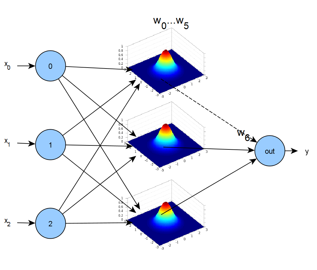
The implementation of the Gaussian mixture model is presented in the code fragment bellow. We have defined an helper object Gaussian that implements a single Gaussian function: Gaussian.f(x) is the function value, Gaussian.df_alpha(x) is the derivative with respect to the parameter  ,
, Gaussian.df_mu(x) the derivative with respect to vector  , and
, and Gaussian.df_sigma(x) the derivative with respect to vector  .
.
import breeze.linalg.{DenseVector => BDV}
import breeze.linalg.{DenseMatrix => BDM}
import breeze.linalg._

/**
 * @author Nodalpoint
 */

class GaussianMixtureModel(inputDim: Int, numGauss: Int)
                                      extends Serializable  with NonlinearModel {
  var n:Int = inputDim
  var m:Int = numGauss
  var dim:Int = m*(n*2+1)


  def eval(w:BDV[Double], x: BDV[Double]): Double = {
    assert(x.size == n)
    assert(w.size == dim)
    var res:Double = 0.0

    for (i<-0 until m){
      var ww:BDV[Double] = w((2*n+1)*i until (2*n+1)*(i+1))
      var alpha:Double = ww(n*2)
      var mu:BDV[Double] = ww(0 until n)
      var sigma:BDV[Double] = ww(n until 2*n)

      res = res + Gaussian.f(x, alpha, mu, sigma)
    }
    return res
  }

  def grad(w: BDV[Double], x: BDV[Double]): BDV[Double] = {
    assert(x.size == n)
    assert(w.size == dim)
    var gper : BDV[Double] = BDV.zeros(dim) // (2n+1)*m
    for (i<-0 until m){
       var ww:BDV[Double] = w((2*n+1)*i until (2*n+1)*(i+1))

       var alpha:Double = ww(n*2)
       var mu:BDV[Double] = ww(0 until n)
       var sigma:BDV[Double] = ww(n until 2*n)

       var alpha_der = Gaussian.df_alpha(x, alpha, mu, sigma)
       var mu_der = Gaussian.df_mu(x, alpha, mu, sigma)
       var sigma_der = Gaussian.df_sigma(x, alpha, mu, sigma)
       gper((2*n+1)*(i+1)-1) += alpha_der
       gper((2*n+1)*i to (2*n+1)*i+ (n-1)) := gper((2*n+1)*i to (2*n+1)*i+(n-1)) +  mu_der
       gper((2*n+1)*i+n to (2*n+1)*i+n+ (n-1)) := gper((2*n+1)*i+n to (2*n+1)*i+n+ (n-1)) + sigma_der

     }
    return gper
  }

  def gradnumer(w: BDV[Double], x: BDV[Double]) : BDV[Double] = {
    var h: Double = 0.000001
    var g:BDV[Double] = BDV.zeros(this.dim)
    var xtemp:BDV[Double] = BDV.zeros(this.dim)
    xtemp = w.copy
    var f0 = eval(xtemp, x)

    for (i<-0 until this.dim){
      xtemp = w.copy
      xtemp(i) += h
      var f1 = eval(xtemp, x)
      g(i) = (f1-f0)/h
    }
    return g
  }

  def getDim(): Int = {
    return dim
  }
}

object Gaussian{
  def exponent(x: BDV[Double], mu: BDV[Double], sigma: BDV[Double]) : Double = {
    var dim:Int = x.length

     var I = BDM.eye[Double](dim)
    for (i<-0 until dim){
      I(i, i) = 1.0 / (sigma(i)*sigma(i))
    }
    var det:Double = -0.5* ((x-mu).t * I * (x-mu))
    var expdet = Math.exp(det)
    return expdet
  }

  def f(x: BDV[Double], alpha: Double, mu: BDV[Double], sigma: BDV[Double]) : Double = {
    var dim:Int = x.length

    var res: Double = 0.0
    var I = BDM.eye[Double](dim)
    for (i<-0 until dim){
      I(i, i) = 1.0 / (sigma(i)*sigma(i))
    }
    var det:Double = -0.5* ((x-mu).t * I * (x-mu))
    var expdet = Math.exp(det)
    res = alpha * expdet

    return res
  }

   def df_alpha(x: BDV[Double], alpha: Double, mu: BDV[Double], sigma: BDV[Double]) : Double = {
     return f(x, 1.0, mu, sigma)
   }

   def df_mu(x: BDV[Double], alpha: Double, mu: BDV[Double], sigma: BDV[Double]) : BDV[Double] = {
      var dim:Int = x.length
      var g:BDV[Double] = BDV.zeros[Double](dim)
      val ex:Double = exponent(x, mu, sigma)
      var sc:Double =  alpha
      for (i<-0 until mu.length){
        g(i) = sc *(1.0 / (sigma(i)*sigma(i)) )*(x(i)-mu(i))*ex
      }

     return g
   }

  def df_sigma(x: BDV[Double], alpha: Double, mu: BDV[Double], sigma: BDV[Double]) : BDV[Double] = {
      var dim:Int = x.length
      var g:BDV[Double] = BDV.zeros[Double](dim)
      val ex:Double = exponent(x, mu, sigma)
      var sc: Double = alpha
      for (i<-0 until mu.length){
        g(i) = (1.0/(sigma(i)*sigma(i)*sigma(i)))* sc *(x(i)-mu(i))*(x(i)-mu(i))*ex
      }

     return g
  }
}
Some test code
We can provide some test code for the nonlinear models we have presented so far, just to check the sanity of the derivatives. You can donwload the code from here: use the sbt utility to create an Eclipse project as descrcibed in this post; then import the project in Eclipse and run, as a Scala application, the NonlinearModelTest.scala file.
import breeze.linalg.{DenseVector => BDV}
import breeze.linalg._

/**
 * @author Nodalpoint
 */
object NonlinearModelTest {
  def main(args: Array[String]) = {
    /**
     * Input dimensionality n = 2
     */
    var n:Integer = 2
    /**
     * Let x be a random data point
     */
    var x: BDV[Double] = BDV.rand[Double](n)
    /**
     * Define one neural network with 2 hidden layers and one
     * Gaussian mixture with two gaussians.
     */
    var nnModel: NonlinearModel = new NeuralNetworkModel(n, 2)
    var gmmModel: NonlinearModel = new GaussianMixtureModel(n, 2)
    /**
     * Get the dimensionality of tunable parameters for each model
     */
    var nnDim: Int = nnModel.getDim()
    var gmmDim: Int = gmmModel.getDim()

    /**
     * Define a random initial set of parameters
     */
    var nnW:  BDV[Double] = BDV.rand[Double](nnDim)
    var gmmW:  BDV[Double] = BDV.rand[Double](gmmDim)

    /**
     * Evaluate the model for input x on parameters nnW
     * nnW[0] weight 1st input to 1st hidden
     * nnW[1] weight 2nd input to 1st hidden
     * nnW[2] weight      bias to 1st hidden
     * nnW[3] weight 1st hidden to output
     */
    System.out.println("Using weights " + nnW)
    System.out.println("On input x " + x)
    System.out.println("NN eval " + nnModel.eval(nnW, x))
    System.out.println("NN grad analytic " + nnModel.grad(nnW, x))
    System.out.println("NN grad numeric " + nnModel.gradnumer(nnW, x))

     /**
     * Evaluate the model for input x on parameters gmmW
     * gmmW[0] 1st gaussian 1st component of mean vector
     * gmmW[1] 1st gaussian 2nd component of mean vector
     * gmmW[2] 1st gaussian 1st component of diagonal covariance
     * gmmW[3] 1st gaussian 2nd component of diagonal covariance
     * gmmW[4] 1st gaussian scale factor alpha
     */
    System.out.println("Using weights " + gmmW)
    System.out.println("On input x " + x)
    System.out.println("GMM eval " + gmmModel.eval(gmmW, x))
    System.out.println("GMM grad analytic " + gmmModel.grad(gmmW, x))
    System.out.println("GMM grad numeric " + gmmModel.gradnumer(gmmW, x))
  }
}
Running the code above we get the following results:
Using weights DenseVector(0.525727523828039, 0.028340085920725233, 0.25861856410832207, 0.4952384746672509, 0.2117473122297735, 0.20716177456458218, 0.871552133260552, 0.6719136810889594)
On input x DenseVector(0.8458565037934767, 0.9182696697451167)
NN eval 0.8553331564886653
NN grad analytic DenseVector(0.09194631898190019, 0.09981777711365018, 0.10870202991824451, 0.6746587663929581, 0.09887970283650667, 0.10734472296537836, 0.11689890944037597, 0.7757189543374099)
NN grad numeric DenseVector(0.0919463053472569, 0.09981776105671969, 0.10870201083701403, 0.6746587664085979, 0.0988796797773972, 0.10734469579887218, 0.11689887724486425, 0.7757189541823806)

Using weights DenseVector(0.15314583219833633, 0.6201623431092302, 0.20563456206912067, 0.057100885706953264, 0.22152119433136153, 0.14306722748581624, 0.28173125185028214, 0.8554151945635102, 0.21623603161511307, 0.3078482411348773)
On input x DenseVector(0.8458565037934767, 0.9182696697451167)
GMM eval 0.002884547772836078
GMM grad analytic DenseVector(1.5034925207399294E-8, 8.391287003499924E-8, 5.064738647533136E-8, 4.3808499722504457E-7, 4.143108728199514E-9, 0.002770440346666426, 0.039268661027813165, 0.0022761295084087773, 0.11559595862351059, 0.00937002870120632)
GMM grad numeric DenseVector(1.5034848366290987E-8, 8.391638078864005E-8, 5.064828764722584E-8, 4.3817813960567165E-7, 4.1429533415016095E-9, 0.0027704397070719977, 0.03926889746925025, 0.0022761264162514394, 0.11559747296148101, 0.009370028700855793)
Notice how close the numerical derivatives vector grad numeric approximates the analytical one grad analytic. That’s a good sign! We can now proceed to define the loss (objective) function. So far we have just scratched the surface of our objective: these nonlinear models and their expressiveness will form the basis of the regression process to be described in the next posts.
Wrap-up & next steps
This post is the preamble for a series of posts concerning nonlinear regression modeling using Scala and Spark.
Up to the current version 1.6.0, Spark MLlib implements only linear regression models, and in these posts we attempt to provide Spark (Scala) code to extend to nonlinear ones. We began with a quick definition of regression and how it can be viewed either as training or fitting or optimizing. We started scratching the subject bottom up, and described a general implementation of what we call a nonlinear model. We have also provided two generic nonlinear models suitable for any regression task, namely feed forward neural network and Gaussian mixture model.
In the next post we will define the nonlinear objective (or loss) function that must be optimized in order to fit (train) the nonlinear model to sample train data – stay tuned!
- Nonlinear regression using Spark – Part 2: sum-of-squares objective functions - October 31, 2016
- How to evaluate R models in Azure Machine Learning Studio - August 24, 2016
- Nonlinear regression using Spark – Part 1: Nonlinear models - February 10, 2016
how to update weights? weights += stepSize*g1 where var (f1, g1) = modelfunRDD.calculate(w) ?
[…] that discusses algorithmic and implementation issues about nonlinear regression using Spark. In the previous post we identified a small window for contribution into Spark MLlib by adding methods for nonlinear […]